When people think about AI hardware, GPU compute is usually the first thing that comes to mind. But in practice, GPUs frequently run into two other problems: the data can't fit, or the data can't be delivered fast enough.
Take a 7B model as an example. "7B" means it has roughly 7 billion parameters. Under typical configurations, full-parameter training on those 7 billion parameters demands over 100 GB of VRAM(GPU memory)— and that number only grows with larger batch sizes or longer inputs. At inference time, however, the same model can, under the right configuration, fit comfortably onto a single 24 GB GPU.
Training and inference use the same model — so why do their memory requirements differ so dramatically? To answer that, we need to untangle three things: what sits in memory during training, what sits in memory during inference, and what roles HBM, host memory, and SSDs each play.
HBM, Host Memory, and SSDs: What's the Difference?
Large model systems commonly use a three-tier storage hierarchy. The difference between the tiers can be summarized in one line: the closer to the GPU, the faster — but also the smaller and more expensive.
| Storage Tier | Intuitive Analogy | Speed | Capacity | Primary Role |
|---|---|---|---|---|
| HBM (VRAM) | The desk in front of a student | Fastest | Smallest | Holds data currently being computed on |
| DRAM (host memory) | A drawer next to the desk | Slower | Larger | Temporarily holds data that won't fit in VRAM but may be needed soon |
| SSD | A bookshelf at the back of the classroom | Slowest | Largest | Stores datasets, training archives, and infrequently used caches |
Under VRAM pressure, weights and optimizer states are offloaded to DRAM / SSD; activations are discarded or recomputed.
Block border color = destination tier. Blocks travel along dashed flow lanes. Toggle to compare training vs. inference flow direction.
Think of the GPU as a student doing homework. The textbook and scratch paper need to be on the desk. Moving them into the drawer or the bookshelf at the back of the room frees up desk space, but you'll have to retrieve them before using them again. The same applies to data involved in GPU computation: ultimately, it has to land in HBM.
Both training and inference make use of these three storage tiers, but they hit different bottlenecks. In simple terms: training usually hits the capacity ceiling first; inference is more often throttled by bandwidth.
Here, bandwidth refers to how much data can be moved per unit of time. How many books the desk can hold is capacity; how many books you can pull out of the drawer per minute is bandwidth. Capacity answers "how much can fit"; bandwidth answers "how fast can data arrive."
Why Training Needs So Much VRAM
Training continuously adjusts the model based on data. So beyond keeping the model itself in memory, the GPU also needs to hold all the intermediate information required to make those adjustments.
There are four main categories:
- Model weights: The parameters the model has already learned.
- Activations: The intermediate results produced as data passes through each layer. They're needed later when computing how to adjust the parameters.
- Gradients: Signals that tell the system which direction to adjust each parameter, and by how much.
- Optimizer states: Records of the direction and magnitude of past adjustments, helping the training process stay stable.
Training is a bit like a student correcting a completed problem. The model weights are the problem-solving method already learned; the activations are the scratch-paper calculations; the gradients are the correction marks from the teacher; and the optimizer states are like a correction log, tracking which direction previous fixes went and by how much. To get the method right, all these materials need to be kept around.
Toggle components below to see how training VRAM grows from 14 GB to 104 GB.
Current VRAM: 104 GB — 7.4× the inference baseline (14 GB).
Inference primarily reads weights; training must hold all four categories of data simultaneously. The larger the model, the more samples processed at once, and the longer the input text, the higher the VRAM usage climbs. This is why a model that can answer questions on a single GPU may still be unable to run full-parameter training on that same card.
There is no universal formula for exactly how much VRAM a given model needs. Numerical precision, batch size, input length, the choice of optimizer, and the training framework all influence the final number. But the order-of-magnitude difference is consistent: the weights of a 7B model take up only a dozen or so gigabytes on their own; add gradients, optimizer states, and activations, and full-parameter training typically pushes the total past 100 GB.
A per-token comparison makes the gap even clearer. Take Llama-3-8B: at inference, a single token's KV Cache costs about 0.25 MB (FP16); during training, the activations a single token produces during the forward pass cost about 8.7 MB (FP16) — roughly 35× the inference per-token cost.
For the same model, training activations per token are dozens of times larger than inference KV Cache.
Llama-3-8B: Training activations per token (8.7 MB) are 35× the inference KV Cache (0.25 MB).
What to Do When VRAM Runs Short
Training systems commonly use three strategies to reduce VRAM pressure:
| Strategy | In Plain Terms | Cost |
|---|---|---|
| Sharding (e.g., ZeRO) | Split the material across multiple desks — that is, multiple GPUs each hold a portion | GPUs need to communicate frequently |
| Offloading | Stash temporarily unused material in a drawer (DRAM) or even the bookshelf (SSD) | You wait for data to be fetched back |
| Activation recomputation | Don't save all the scratch paper (activations); recompute them when needed | Extra computation and longer training time |
None of these methods makes data disappear. They simply trade more communication, data movement, or recomputation for lower VRAM usage.
Toggle strategies below to watch VRAM pressure drop while the cost rises. Data doesn't disappear.
VRAM pressure is at 100%. Enable any strategy to trade communication, transfer, or recomputation for VRAM.
During training, the system also periodically saves checkpoints — writing the current weights and optimizer states to the SSD. It's like a student saving progress after finishing each section of homework: even if the computer suddenly loses power, they won't have to start over from the first problem. Checkpoints are primarily for fault tolerance, not for speeding up the current computation step.
Why Inference Cares More About Bandwidth
Inference uses a trained model to generate answers. There's no need to compute gradients or maintain optimizer states, so far fewer types of data live in memory. Beyond model weights, the single most important item is the KV Cache.
What Is the KV Cache?
When a large model generates a response, it writes token by token. A token is the small unit the model uses to segment text — it could be a character, part of a word, or a punctuation mark. When generating the next token, the model needs to reference all preceding input and previously generated content.
If the model had to recompute the entire preceding text from scratch for every new token, it would waste enormous amounts of compute. The KV Cache stores the intermediate results already computed for the preceding text, letting subsequent generation steps reuse them directly. What it stores are the computational outcomes of processing the text — the original chat text remains part of the input.
Think of the KV Cache as the notes a student takes while reading a long passage. Without notes, every sentence of the answer would require rereading from page one. With notes, the student can jump straight to the key points already summarized. The KV Cache stores exactly this kind of "notes" for later computation.
This approach cuts redundant computation, at the cost of VRAM. The longer the context and the more concurrent users, the larger the KV Cache grows.
How big is the KV Cache for a single token, concretely? Under FP16 precision:
| Model | Per-Token KV Cache (estimated) |
|---|---|
| Llama-2-7B | ~1.0 MB |
| Llama-3-8B | ~0.25 MB |
| Llama-3-70B | ~0.63 MB |
| DeepSeek-V3 671B (MoE) | ~0.5–1 MB |
| GPT-3 175B | ~14.0 MB |
Among models of similar parameter counts (7–8 billion), Llama-3-8B uses only 1/4 of Llama-2-7B's per-token KV Cache. The reason: Meta introduced GQA (Grouped-Query Attention) in Llama-3, compressing the number of Key and Value heads to one quarter.
DeepSeek-V3 takes this further. Despite its massive parameter count (671B), it uses MLA (Multi-head Latent Attention), which compresses KV into low-rank latent vectors for storage, bringing per-token KV usage down to 1/10 to 1/4 of mainstream dense models. This is the architectural reason behind DeepSeek's official claim of "reducing KV Cache cost to 1/10 of the previous generation."
In contrast, GPT-3 175B predates GQA — without KV head compression, a single token costs 14 MB of KV Cache. This is why long-context inference was nearly infeasible on older architectures.
Switch architectures to watch the number of KV heads — and the per-token cache — shrink step by step.
Lit cells = KV groups actually stored. MHA compresses the KV of 8 query heads into 8.
MHA:Every query head has its own Key and Value — no compression.
MHA is the baseline: each head stores KV independently — cache grows fastest under long context.
These numbers multiply quickly with context length:
| Model | 8K Context | 32K Context | 128K Context |
|---|---|---|---|
| Llama-3-8B | ~2 GB | ~8 GB | ~32 GB |
| Llama-3-70B | ~5 GB | ~20 GB | ~80 GB |
| GPT-3 175B | ~112 GB | ~448 GB | ~1.8 TB |
On an H100 with 80 GB of VRAM, running Llama-3-70B at 128K context means the KV Cache alone nearly fills the card. That is exactly why DeepSeek, Mooncake, vLLM, and others are racing to implement KV compression and tiered storage — in long-context scenarios, the KV Cache is the number-one VRAM killer.
Drag the slider to change context length. Watch KV Cache grow linearly and break through the 80 GB H100 VRAM ceiling.
At 32K context: both models' KV Cache fit within 80 GB.
Why the GPU Ends Up Waiting for Data
The generation phase is typically called Decode. For every token the model generates, it must read a large volume of model weights as well as the accumulated KV Cache.
If this data can't be fed to the compute units fast enough, the GPU sits idle — even if it has spare compute capacity. At this point, speed is determined by how much data can be read from VRAM per second. This is the memory bandwidth bottleneck.
Imagine a student who writes quickly but has to flip through notes before each word. If the notes arrive too slowly, they spend most of their time just waiting. How fast the student writes corresponds to GPU compute; how fast the notes reach their hand corresponds to memory bandwidth.
Each generated token re-reads all weights and the KV Cache. If data arrives too slowly, the GPU just waits.
Compute is fast, but every token re-reads all weights + KV Cache. If bandwidth can't keep up, the GPU stalls idle. This is why inference is bandwidth-bound.
"Training hits the capacity ceiling; inference hits the bandwidth ceiling" is a useful rule of thumb, not a law that holds for every workload. Short inputs, high-concurrency batch processing, or different model architectures can shift the importance of compute, capacity, and bandwidth. But for common large-model training and token-by-token generation, it explains most of what you'll see.
What Happens When the KV Cache Won't Fit
Inference systems also tier their data across storage layers:
| Storage Tier | What Inference Typically Places Here |
|---|---|
| HBM (VRAM) | Model weights and the KV Cache for actively generating responses |
| DRAM (host memory) | KV Cache for sessions that are temporarily inactive but likely to resume soon |
| SSD | Cache for sessions unused for a longer period but still worth reusing |
The system prioritizes keeping data for the current request in HBM, while moving less urgent data to host memory or SSD. It's like a student keeping the notes they're actively using on the desk, recently used ones in the drawer, and long-unused ones back on the bookshelf. When a request becomes active again, the system retrieves the corresponding cache.
Mooncake (from Moonshot AI / Kimi) is a public example. It organizes GPU VRAM, host memory, and SSDs into a larger KV Cache pool, aiming to reduce redundant computation while meeting latency requirements. Inference frameworks like vLLM and SGLang are also building similar tiered caching capabilities.
SSDs offer large capacity at low cost, but their speed is far below HBM. They're good for expanding the range of reusable caches but can't directly substitute for VRAM. The system needs to prefetch data and deliver it to HBM before the GPU needs it. If the prediction is off or the transfer is too slow, caching can actually slow generation down.
Click a request to make it the active generation. The system promotes its KV Cache back into HBM, evicting the least-recently-used block down a tier if needed — like clearing space on your desk.
When HBM fills up, the least-recently-used cache drops to DRAM or SSD; when a request becomes active again, it's promoted back. Prefetch must arrive before the GPU needs it — or generation stalls.
Why "Cache Hit" Pricing Is Much Cheaper
Once you understand the KV Cache, the "cache hit" and "cache miss" entries in vendor pricing tables become much easier to parse.
A single inference pass can be roughly divided into two stages:
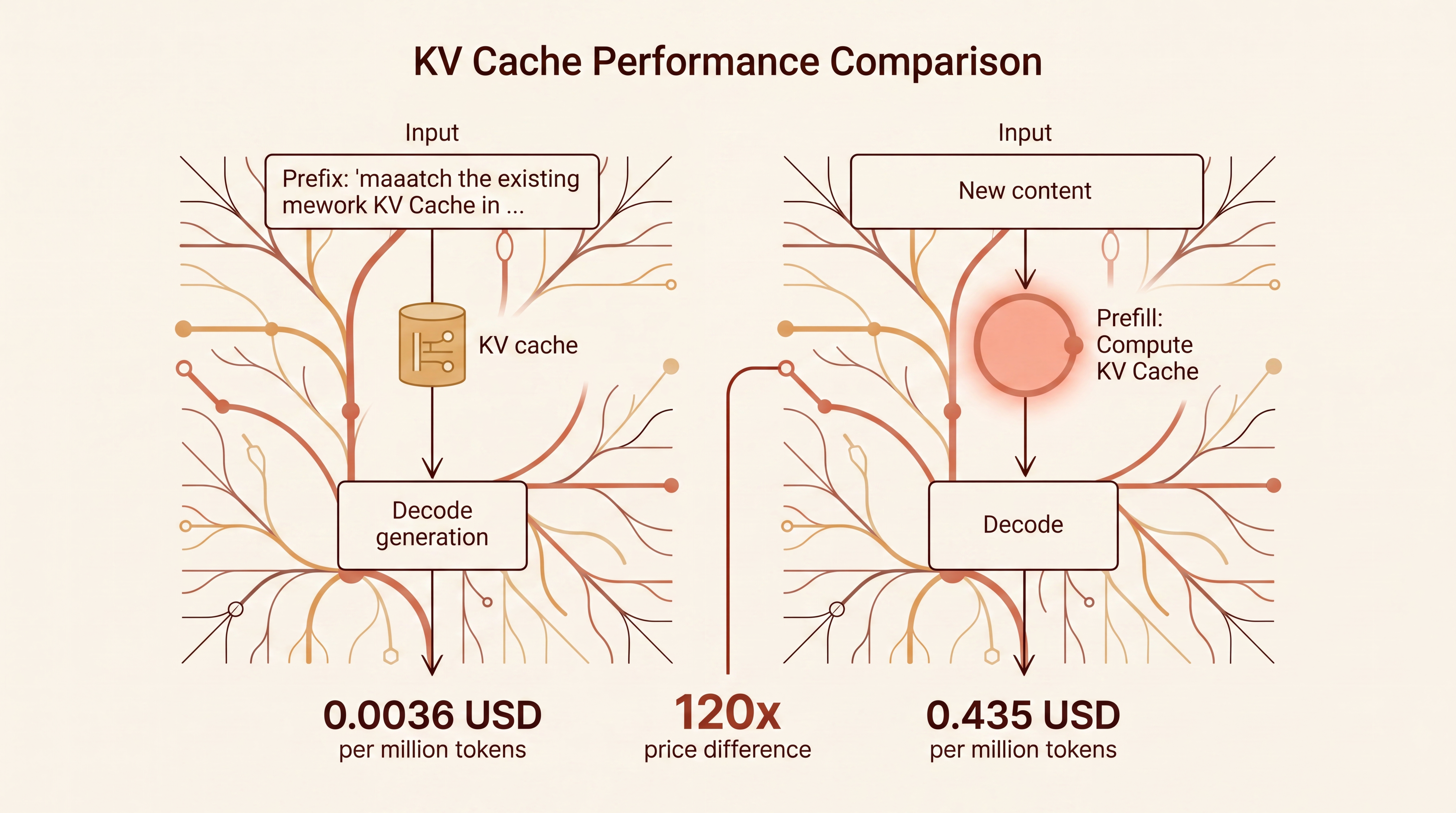
- Prefill: Read the entire input and compute its KV Cache — like reading a passage for the first time and taking notes.
- Decode: Use the previously computed results to generate tokens one by one — like writing an answer while consulting the notes.
If a new request starts with content identical to something previously processed — the same system prompt or the same long document, for instance — the system can directly reuse the already-saved KV Cache. The reused portion skips Prefill entirely, only needing to read the cache, which makes it cheaper.
A cache hit is like getting a second test paper that reuses the same reading passage. The passage hasn't changed, so the earlier notes still apply; only the new questions need fresh work. A cache miss is like getting an entirely new passage — the student has to read it and take notes all over again.
As of July 2026, in DeepSeek's official pricing, V4-Pro's cache-hit price for input is $0.003625 per million tokens, while the cache-miss price is $0.435 per million tokens — a 120x difference. The prices may change over time, but the mechanism behind the gap won't shift with the pricing table: cache hits eliminate redundant computation.
On a cache hit, the system only needs to read the existing KV Cache. On a cache miss, the system must recompute the entire input's KV Cache from scratch. The 120x price gap is essentially the cost difference between "reading from cache" and "computing everything again" — once you understand this, you will know when to reuse system prompts and why to place long documents at the front.
Switch hit/miss, drag the slider to move the divergence point, and watch Prefill/Decode and the price shift.
In hit mode, the first 15 tokens skip Prefill — only a cache read.
Reused prefix 15 / 20 tokens — this part skips Prefill and only reads cache. Compute saved ≈ 75%.
Two common points of confusion are worth calling out.
First, the cache only reduces the cost of the matched portion of the input. Output still has to be generated token by token by the model — it doesn't become free just because the input hit the cache.
Second, cache matching requires a prefix match. "Roughly the same meaning" doesn't count as a hit. The system compares starting from the beginning of the input; the matching prefix portion can be reused, and computation resumes from the first point of divergence.
For example, if the first 10 pages of two handouts are identical but page 11 onward differs, the notes for those first 10 pages can be reused, and only page 11 onward needs to be re-processed.
This is why, when using APIs that support prefix caching, it's generally better to place the fixed system prompt and long documents at the front and the variable questions at the back — that arrangement is more likely to hit the cache. Always consult the vendor's documentation for the exact matching rules. DeepSeek's disk cache guide, for instance, explicitly states that caching operates on prefix units and follows a best-effort approach — no guarantee of a hit every time.
Training vs. Inference: A Side-by-Side Summary
| Dimension | Training | Inference |
|---|---|---|
| Primary task | Modify model parameters | Generate answers using existing parameters |
| What sits in memory | Weights, activations, gradients, optimizer states | Weights, KV Cache |
| Per-token memory cost (8B-class model) | ~8.7 MB (activations) | ~0.25 MB (KV Cache) |
| Typical bottleneck | Too much data — VRAM can't fit it all | Data reads aren't fast enough; can also hit capacity limits under long context and high concurrency |
| Role of host memory and SSD | Store datasets, checkpoints, and offloaded training data | Store KV Cache that's temporarily unused but may be reused |
| Common optimization strategies | Sharding, offloading, recomputation | Cache reuse, tiered storage, compression, and prefetching |
Switch modes to see how the two stages differ in task, memory, bottleneck, and optimization.
Modify model parameters so the model learns.
Data demand is ~1.5× VRAM capacity — the overflow is the bottleneck.
Memory bandwidth fills only ~40% of what the GPU needs — compute starves. Capacity can also bind under long context or high concurrency.
Store datasets, checkpoints, and offloaded training data.
Training optimizations trade more communication and compute for less VRAM.
Many training-side optimizations aim to reduce VRAM usage by spending more communication and compute. Many inference-side optimizations aim to cut redundant computation through caching and get data to the GPU in time.
Closing Thoughts
An AI system is not just a compute resource. Whether a model can run at all, how fast it responds, and why APIs are priced the way they are — all of these are tied to memory capacity, memory bandwidth, and the movement of data between storage tiers.
For now, HBM still handles the most latency-sensitive work, while host memory and SSDs serve to expand capacity and lower cost. How much work the latter two can offload from HBM depends on whether the cache hits and whether data can be fetched back before the GPU needs it.
This is why, alongside compute figures, each new generation of AI chips emphasizes HBM capacity and bandwidth. Peak GPU compute only states the theoretical ceiling; if the data supply can't keep up, real-world utilization will never reach it.